
This is a short and temporary tutorial on Fractal Rock Insights Advertising Spend Analysis and Optimization Platform.
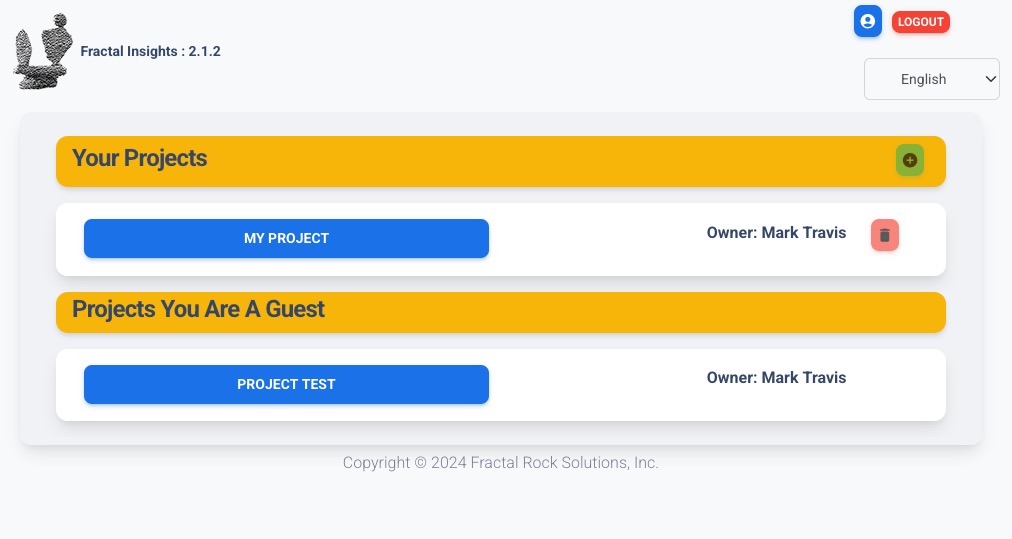
The first thing you will see when you log in is the Projects page. If you have authority to create your own projects, they will show up in the top section titled “Your Projects.” If someone else has created a project, they can add you as a guest to their project and it will show up in the second section titled “Projects You Are A Guest.”
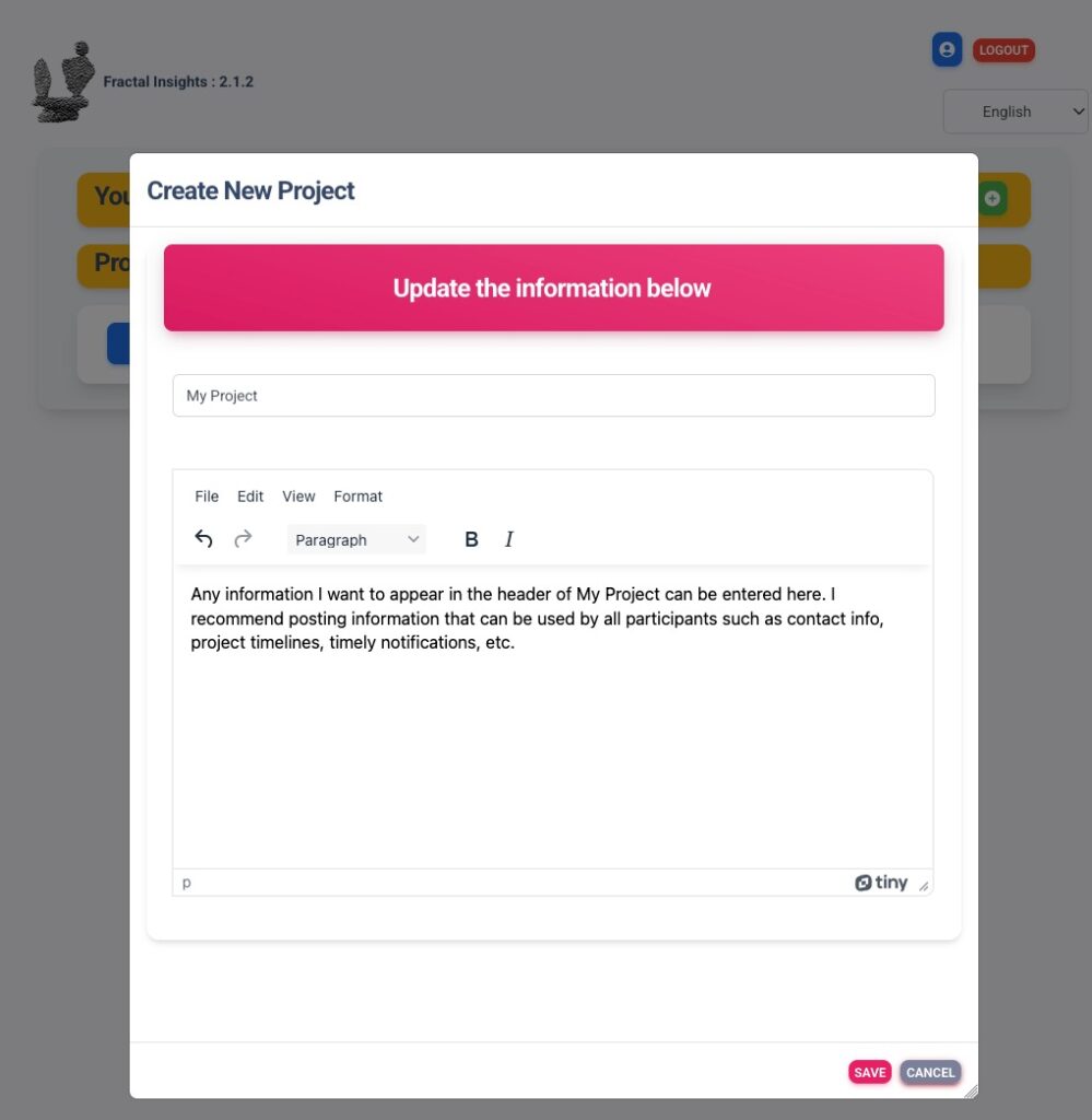
If you have authority to create a project, you can create one by clicking on the green “+” symbol on the right hand side of the “Your Projects” banner. This will bring up the following dialog where you can enter a project name and any additional information about the project you wish to publish.
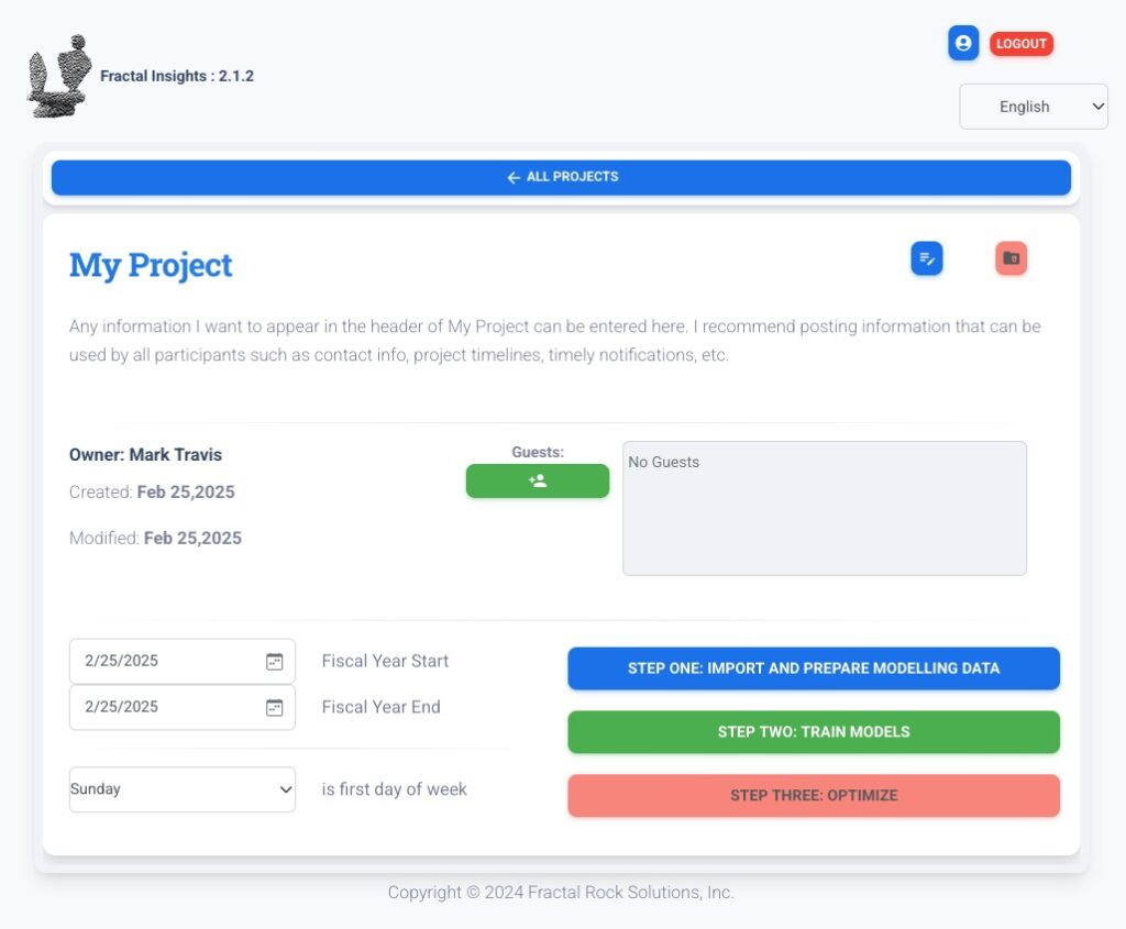
Once you create a new project, you will see the project’s home page. The information you entered on creation will appear at the top. Every person who has access to this project will start at this home page. The first thing you should do is enter the Fiscal Year Start and Fiscal Year End. You can load adverting impressions and run adstocks and rollup columns without setting the FY start and end dates, but as soon as you load spending, checks and balances of advertising impressions and spending occur and the system will reject any spending with no impressions or impressions with no spending. If you have set the proper FY and you get spending or impressions mismatch errors, these must be fixed before you can continue.
IMPORTANT NOTE! Always use the bars at the top of each page to navigate backwards and forwards to different Workbench areas. If you use your browsers forward and backward button, you’ll likely end up on some other webpage you’ve visited in the past. If you click on the “refresh” button, you may end up back at the projects page, but that’s ok as all work is usually saved at the time of the operation.
SECOND IMPORTANT NOTE! Nothing in this system is ever deleted immediately. Instead, everything that is “deleted” is actually archived. This provides a way to “undo” as well as provide an audit trail to show who did what and at what time. This is very important if multiple people are working on the system and you need to revert to a prior project state. (Or point the finger at someone for deleting someone else’s work! 😊)
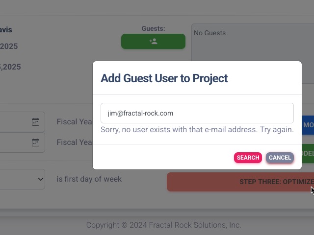
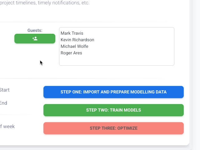
You can also add other participants to your projects on this panel. You must add them based on their registered e-mail address. The participant must already be active on FRS Insights and you must know the e-mail address of the participant you want to add. No, you can’t choose from a drop-down list. This process is designed to maintain privacy of participants in a shared environment. If you type an e-mail of a non-registered user you will get an error message to that effect.
Otherwise, the name of the person will show up to the right of the Guests Add button.
Loading Advertising Data and Preparing Impressions for Modeling
Look for instructions on the Advertising Impressions and Spending Workbench in a future iteration of this guide.
Modeling The Advertising Response Environment
To create or view advertising models, click on “STEP TWO: TRAIN MODELS” from the project home page.
The next page allows you to create models from the advertising data (future tutorial addition); create models with your own data; or work with existing models. If you create a model using your own data (vs the advertising data loaded in the prior “STEP ONE” process, it will not be used in the calculations or optimizations. This allows you to upload your own data and play around with theories or hunches without affecting the official models. Eventually one will be able to selectively import project data to an “outside” model, but for now that is not available.
If you want to create your own, external model, click on the green plus symbol at the top of the page next to “Model:”
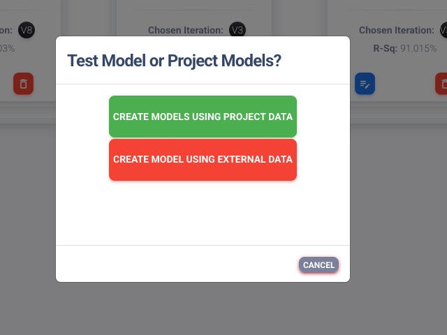
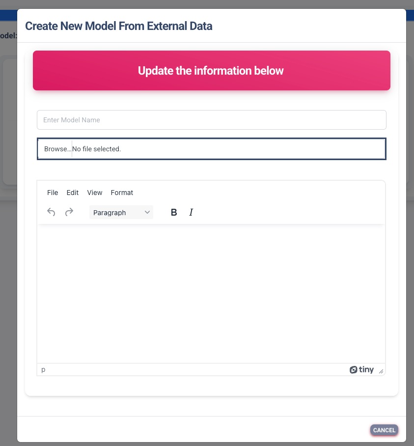
Choose “CREATE MODEL USING EXTERNAL DATA.” This will pop-up a dialog to upload a .CSV file from your computer. Like the Project creation panel, you can make notes on this file here. If you don’t supply a name for the model, it will inherit the name of the .CSV file.
Once the file is loaded, the Modeling Workbench appears. This is the same page as working with your data or working with Advertising data. If you want to review or change notes for this model, click on the downward facing chevron symbol at the top of the page opposite the model name. It will expand this section and you can edit or change the notes you made on the Model when it was created. Click on the blue button that appears once the section expands to bring up the editor.
The left hand sub-panel contains information about the file, and the training parameters. All parameters which control training are in this panel. The “Filename” contains a button that allows anyone with access the ability to download the .CSV used in this model. This could be useful if one wants to create a macro-enabled Excel worksheet, and download a trained model as an Excel Custom Function to run what-if scenarios that aren’t baked into the platform at this time. Training available on request.
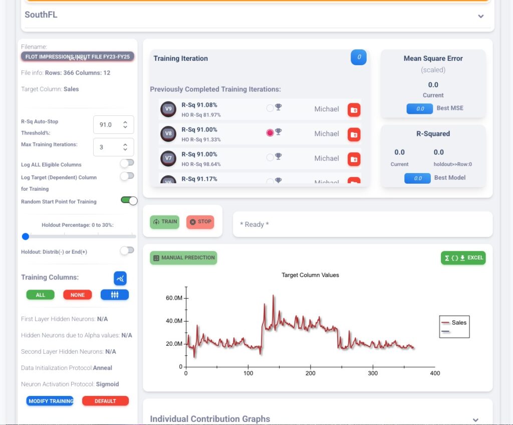
Next you will see the number of rows and columns loaded from the .CSV file. If you upload your own data, the dependent variable MUST be loaded as the most far-right column. In this example, the predicted/dependent variable is “Sales.”
In order to not waste compute on needless over-iterations of training, the defaults have been chosen to give a reasonable environment to come up with an acceptable model. If you want a higher or lower R-Squared, more training iterations, logging of independent or dependent variables, random starting points, holdout % and whether holdout is randomly distributed or always taken from the last rows of the dataset, modify them in this panel.
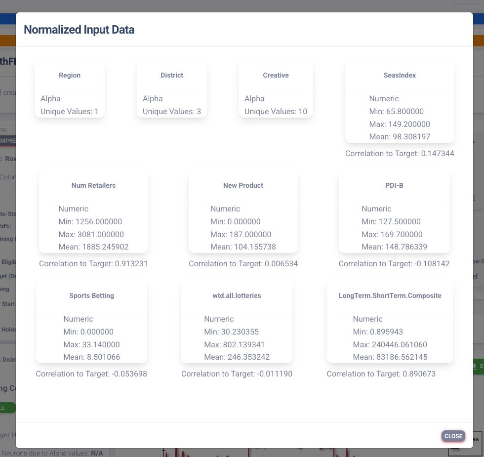
In the “Training Columns” section, there is a blue button with a magnifying glass and stairstep graphic. Click on this button to see meta data on the data that was uploaded to this model. This panel will eventually grow in functionality to show co-variance, co-linearity, and other data points to show which columns may or may not be useful for getting the appropriate and best results from the model.
Back at the main Modeling Workbench, you can select which columns you want to use for training, and also override the neural network training parameters. Don’t play with these unless you understand how that effects the model.
One thing to understand about using AI vs other statistical methods such as Regression, is that AI can memorize your model exactly and precisely with a very high R-Squared. The problem is, this is not what you want!! If you used that model on another dataset, you would most likely get a pretty low R-Squared. You want to get a reasonably responsive model that acknowledges the large and small swings in the Target variable without also following the extremes. This is known as “over-fitting”
When one is getting their Phd in a subject, they must read and understand the subject from many different sources, so that they can determine how real-life is responding to theory. If they only read one school of thought, then they would be biased completely that direction. With a hammer, everything is a nail! This person would be “over-fitted.”
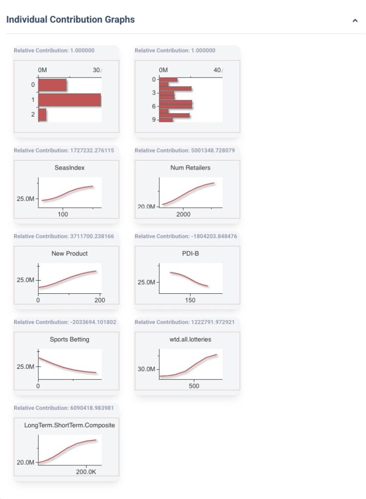
This biggest sign that you have over-fitted the data is if any of the charts in the “Individual Contribution Graphs” show a kinked line like an upside down “V” or something like that. What you want to see is a nice upward or downward sloping “S-Curve,” or even a flat line. Note: “Individual Contribution Graphs” are populated as soon as a model is selected from the “Training Iteration” section at the top of the Workbench. Select the downward facing chevron to expand this section so that you can see the charts.
Back to the training columns, you can either select “All”, “None”, or select from a list to select the training columns you want to use in your model. Or, you can select the columns by clicking the check box at the top of each column. Or you can use both methods.
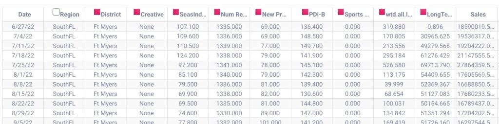
Once selected they will show in the left hand column. You can remove the column from training using the red trash can icon or unchecking the check box in each column. (No, it doesn’t delete the data, just removes it from training the model.) Also available is to individually assign a Log or ArcTan to each individual column by clicking on the blue Greek Summation symbol in each column’s box. It will change the title to show the Log or ArcTan operation.
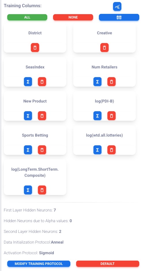
Back to the main panel:
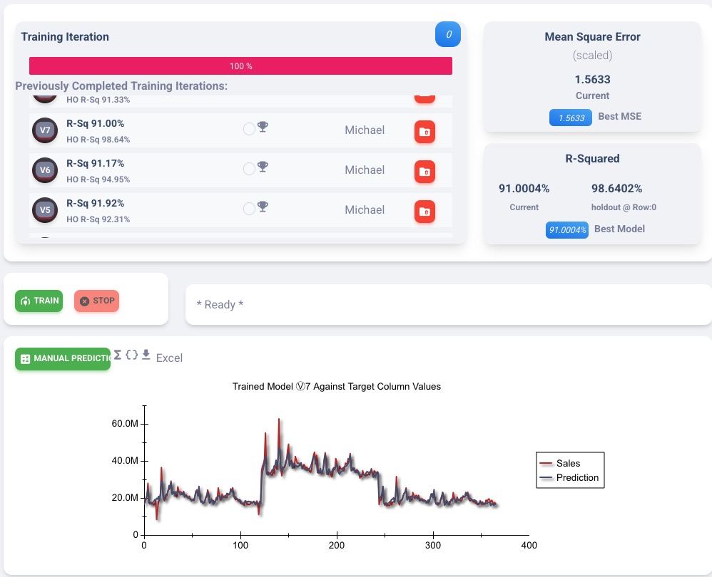
This is where all of the action happens after you select the columns you want to train with and set all of the training parameters to your satisfaction. The first time you create a model, there will not be any rows in the “Previously Completed Training Iterations:” section. Click the green “Train” button to create a new Model Training Iteration. You can create as many of these as necessary. When you find the training iteration(s) you like, you can delete the ones you don’t like by clicking the red icon.
Once you have a model that you deem is as good as you need, click in the circle next to the trophy icon. That will set this training iteration as the official configuration for this model. This is only important for models that directly use the advertising data and will be used in the subsequent Optimization “STEP THREE” of the project. If it’s just a model that you are playing around with using your data, this won’t be of great importance except as a bookmark for your future reference.
Mean Square Error is a unit-less measure and is useless to compare to other models/data. It is only a measurement useful to the current model. R-Squared is probably a better measurement. A good R-Square is something north of 80% and south of 94%. Anything above 94% is probably over-fitting. Anything under 80% is likely leaving too much nuance out of the model. The sweet spot is right around 89 to 91.
To view the results of any of the Training Iterations, click on the Vx button to the far left of each training iteration. This will load that training iteration including all of the training parameters, and graph the model prediction for that training iteration against the target variable (dependent.) The title of the graph will also show which Training Iteration is selected. You can use the selected Training Iteration as a starting point to tweak training settings for another training.
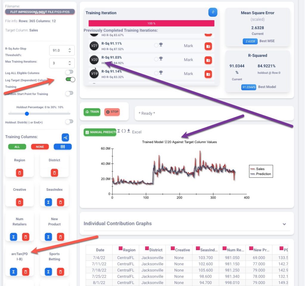
You can download the selected Training Iteration for this model by clicking on the green Excel button at the top right corner of the main chart. This will download a Visual Basic module that you can import into Excel and run against similar values.
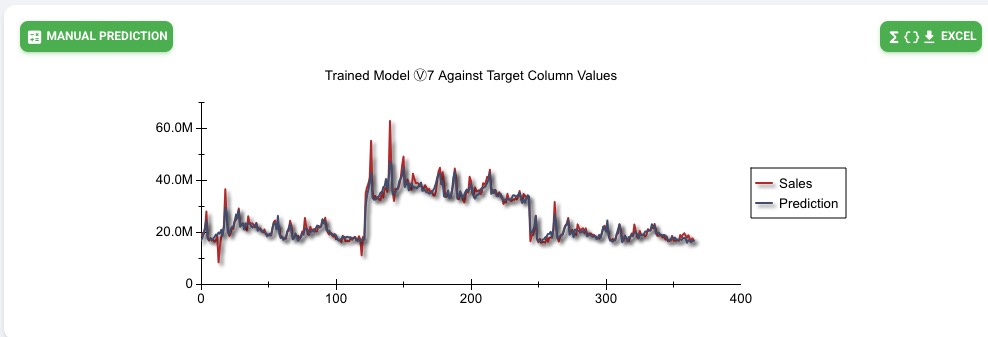
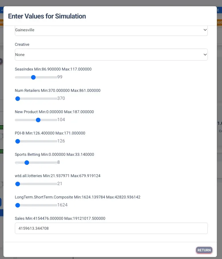
Finally, if you want to see how this Training Iteration for this model responds to the underlying data, you can click on the “Manual Prediction” button at the upper left and a dialog box will appear allowing you to set the values to see the affect on the dependent variable displayed at the bottom of the dialog.
Running The Optimization And Analyzing The Results
This section under construction.